1.1.1 Linear equations and inequalities; solving and graphing
A linear equation is an equation in which the highest power of the variable is always 1. It is also known as a one-degree equation. When this equation is graphed, it always results in a straight line. This is the reason why it is termed as a ‘linear equation’. There are linear equations in one variable, in two variables, in three variables, and so on. The standard form of a linear equation in one variable is of the form Ax + B = 0. An equation of the form Ax + By = C is called a linear equation in two variables. A few examples of linear equations are 5x + 6 = 1, 42x + 32y = 60, 7x = 84, etc.
A linear equation in one variable is an equation in which there is only one variable present. It is of the form ax + B = 0, where a and b are any two real numbers and x is an unknown variable that has only one solution. For example, 9x + 78 = 18 is a linear equation in one variable.
A linear equation in two variables is of the form ax + by + c = 0, in which A and B are the coefficients, C is a constant term, and x and y are the two variables, each with a degree of 1. For example, 7x + 9y + 4 = 0 is a linear equation in two variables.
We can solve a linear equation in one variable by moving the variables to one side of the equation, and the numeric part on the other side. For example, x – 1 = 5 – 2x can be solved by moving the numeric parts on the right-hand side of the equation, while keeping the variables on the left side. Hence, we get x + 2x = 5 + 1. Thus, 3x = 6. This gives x = 2.
When we graph linear equations, it forms a straight line. In order to graph an equation of the form, Ax + By = C, we get two solutions that are corresponding to the x-intercepts and the y-intercepts. We convert the equation to the form, y = ax + b. Then, we replace the value of x with different numbers and get the value of y which creates a set of (x, y) coordinates. These coordinates can be plotted on the graph and then joined by a line.
|
Example 1 Solve for x: 3x – 12 = 0 Solution 3x – 12 = 0 3x = 12 x =4 |
Example 2 Solve for x: 5 (2x – 1) = 4 (3 x – 2) Solution 5 (2x – 1) = 4 (3 x – 2) 10x – 5 = 12 x – 8 10x – 12x = -8 + 5 -2x = – 3 x = 3/2
|
Example 3 Solve for x: 4(x + 5) = 3(x – 2) – 2(x + 2) Solution 4 (x + 5) = 3 (x – 2) – 2 (x + 2) 4x + 20 = 3x – 6 -2x -4 4x -3x + 2x = -20 -6 -4 3x = -30 x = -10 |
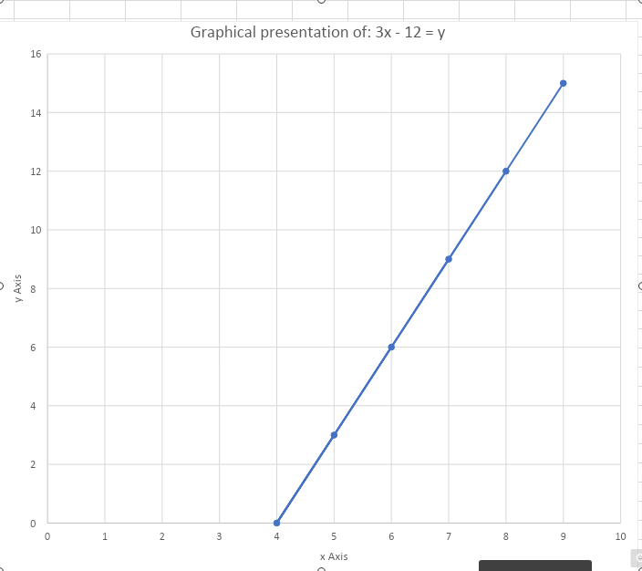
From the above illustrations draw graphs from the above equation 3x – 12 = y.
assume y coordinates to be as follows
| Y | 3 | 6 | 9 | 12 | 15 |
Example 1
| x | 5 | 6 | 7 | 8 | 9 |
| y | 3 | 6 | 9 | 12 | 15 |
1.1.2 Simultaneous equations and inequalities; solving and graphical presentation.
Simultaneous equations are two or more algebraic equations that share common variables and are solved at the same time (that is, simultaneously). For example, equations x + y = 5 and x – y = 6 are simultaneous equations as they have the same unknown variables x and y and are solved simultaneously to determine the value of the variables. We can solve simultaneous equations using different methods such as substitution method, elimination method, and graphically.
Solving simultaneous equations.
Simultaneous equations can have no solution, an infinite number of solutions, or unique solutions depending upon the coefficients of the variables. We can also use the method of cross multiplication and determinant method to solve linear simultaneous equations in two variables. We can add/subtract the equations depending upon the sign of the coefficients of the variables to solve them. To solve simultaneous equations, we need the same number of equations as the number of unknown variables involved.
Simultaneous equation rules
To solve simultaneous equations, we follow certain rules first to simplify the equations. Some of the important rules are:
- Simplify each side of the equation first by removing the parentheses, if any.
- Combine the like terms.
- Isolate the variable terms on one side of the equation.
- Then, use the appropriate method to solve for the variable.
Solving simultaneous equations by elimination method
To solve simultaneous equations by the elimination method, we eliminate a variable from one equation using another to find the value of the other variable. Let us solve an example to understand find the solution of simultaneous equations using the elimination method. Consider equations 3x – 2y = -2 and 5x – 6y = 10. We have
3x – 2y = -2 — (1)
and 5x – 6y = 10 — (2)
Here, we will eliminate the variable y, so we will multiply equation (1) by 3 to make both coefficients similar. So, we have
[3x – 2y = -2] *3
5x – 6y =10
Simplify
9x – 6y = -6
5x -6y = 10
Subtract the two equations to eliminate y
9x – 6y = -6
5x – 6y = 10
4x = -16
Solve for the remaining variable, x = -4
Substitute x = -4 in the original equations (3 * -4) – 2y = -2
Solve for y -12 – 2y = -2
-2y = 10
y = -5
So, the solution of the simultaneous equations 3x – 2y = -2 and 5x – 6y = 10 using the elimination method is x = -4 and y = -5
Solving simultaneous equations by substitution method
To solve simultaneous equations by the substitution method, we make one coefficient of the first equation the subject of the formula, then substitute it in the second equation. Let us solve an example to understand find the solution of simultaneous equations using the substitution method. Consider equations 3x – 2y = -2 and 5x – 6y = 10. We have
3x – 2y = -2
5x – 6y = 10
make x subject of the formula x = (2 + 2y)/3
Substitute x in equation II 5[ (-2 +2y)/3 ] – 6y = 10
solve the equation 3 (5[ (-2 + 2y)/3 ] ) – 3(6y) = (10) 3
5(-2 + 2y) – 18y = 30
– 10 + 10y – 18y = 30
-8y = 40
y= -5
find x 3x – 2y = -2
3x -( 2)(-5) = -2
3x = -12
x = -4
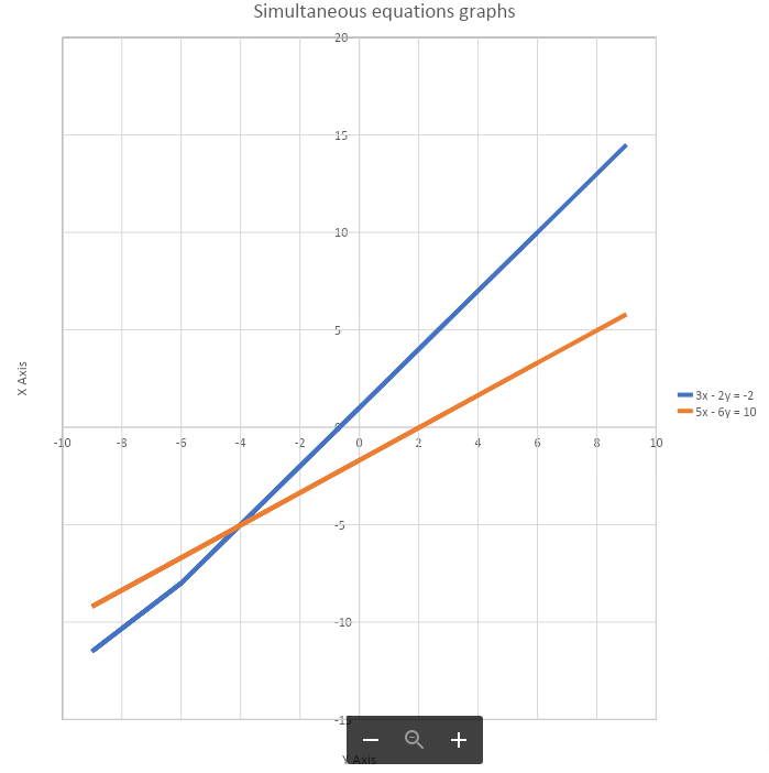
Solving simultaneous equations graphically
Plot the lines on the coordinate plane and then find the point of intersection of the lines to find the solution. Consider simultaneous equations 3x – 2y = -2 and 5x – 6y = 10. Now, find two points (x, y) satisfying for each equation such that the equation holds.
3x – 2y = -2
| X | -9 | -6 | -3 | 0 | 3 | 6 | 9 |
| Y | -11.5 | -8 | -3.5 | 1 | 5.5 | 10 | 14.5 |
5x – 6y = 10
| X | -9 | -6 | -3 | 0 | 3 | 6 | 9 |
| Y | -9.2 | -6.7 | -4.2 | -1.7 | 0.8 | 3.3 | 5.8 |
1.1.3 Quadratic equations; solving and graphing.
A quadratic equation is an algebraic equation of the second degree in x. The quadratic equation in its standard form is ax2 + bx + c = 0, where a and b are the coefficients, x is the variable, and c is the constant term. The first condition for an equation to be a quadratic equation is the coefficient of x2 is a non-zero term(a ≠ 0). For writing a quadratic equation in standard form, the x2 term is written first, followed by the x term, and finally, the constant term is written. The numeric values of a, b, c are generally not written as fractions or decimals but are written as integral values.
Types of Quadratic Equations
1. Complete Quadratic Equation ax2 + bx + c = 0, where a ≠ 0, b ≠ 0, c ≠ 0
2. Pure Quadratic Equation ax2 = 0, where a ≠ 0, b = 0, c = 0
roots of quadratic equations
The roots of a quadratic equation are the two values of x, which are obtained by solving the quadratic equation. These roots of the quadratic equation are also called the zeros of the equation. For example, the roots of the equation x2 – 3x – 4 = 0 are x = -1 and x = 4 because each of them satisfy the equation. i.e.,
- At x = -1, (-1)2 – 3(-1) – 4 = 1 + 3 – 4 = 0
- At x = 4, (4)2 – 3(4) – 4 = 16 – 12 – 4 = 0
Methods of solving quadratic equations
a.) Factorization method
In this method, we factorize the equation into two linear factors and equate each factor to zero to find the roots of the given equation.
Step 1: Given Quadratic Equation in the form of ax2 + bx + c = 0.
Step 2: Split the middle term bx as mx + nx so that the sum of m and n is equal to b and the product of m and n is equal to ac.
Step 3: By factorization we get the two linear factors (x + p) and (x + q)
ax2 + bx + c = 0 = (x + p) (x + q) = 0
Step 4: Now we have to equate each factor to zero to find the value of x.
solve the following equation by factorisation.
u² – 5u -14 = 0
split the middle term bx (5u) as mx + nx so that the sum of m and n is equal to b (2, -7)
and the product of m and n is equal to ac (2 * -7 = -14. i.e. , 1 (a) * -14 (c)
Therefore, u² – 5u – 14 = 0
u² + 2u – 7u -14 = 0
u( u + 2 ) – 7( u + 2 ) = 0
( u – 7 ) ( u + 2 ) = 0
u1 = 7, u2 = -2
b.) Quadratic formula.
In this method, we can find the roots by using quadratic formula. The quadratic formula is
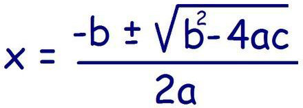
where a, b and c are the real numbers and b2 – 4ac is called discriminant.
To find the roots of the equation, put the value of a, b and c in the quadratic formula.
EXAMPLE I
Solve the following quadratic equation using the quadratic formula: u2 – 5u – 14 = 0
solution:
u = 5 ± √-52 – (4 * 1 * -14)
2 * 1
u = 5± √81
2
u1 = -2 , u2 = 7
solving quadratic equations graphically.
The graph of a quadratic function is a parabola, which is a “u”-shaped curve: A coordinate plane. The x- and y-axes both scale by one. The graph is the function x squared.
solve the following equation graphically: y= x2
| x | -3 | -2 | -1 | 0 | 1 | 2 | 3 |
| y | 9 | 4 | 1 | 0 | 1 | 4 | 9 |

1.1.4 The function y=ex.
An exponential function is a mathematical function of the following form: f ( x ) = a x. where x is a variable, and a is a constant called the base of the function. The most commonly encountered exponential-function base is the transcendental number e , which is equal to approximately 2.71828
One of the popular exponential functions is f(x) = ex, where ‘e’ is “Euler’s number” and e = 2.718….If we extend the possibilities of different exponential functions, an exponential function may involve a constant as a multiple of the variable in its power. i.e., an exponential function can also be of the form f(x) = ekx. Further, it can also be of the form f(x) = p ekx, where ‘p’ is a constant.
exponential graph.
Exponential graph: y = ex
| X | -2 | -1 | 0 | 1 | 2 |
| Y | 0.14 | 0.37 | 1 | 2.72 | 7.34 |

1.1.5 Application of errors; absolute/relative
Absolute Error
Absolute error is the difference between measured or inferred value and the actual value of a quantity. The absolute error is inadequate due to the fact that it does not give any details regarding the importance of the error. While measuring distances between cities kilometers apart, an error of a few centimeters is negligible and is irrelevant. Consider another case where an error of centimeters when measuring small machine parts is a very significant error. Both the errors are in the order of centimeters but the second error is more severe than the first one.
Absolute Error = Actual Value – Measured Value
Absolute error example.
For example, 24.13 is the actual value of a quantity and 25.09 is the measure or inferred value, then the absolute error will be:
Absolute Error = 25.09 – 24.13
= 0.86
Relative Error.
Relative Error = Absolute Error / Known Value
For example, a driver’s speedometer says his car is going 60 miles per hour (mph) when it’s actually going 62 mph. The absolute error of his speedometer is 62 mph – 60 mph = 2 mph. The relative error of the measurement is 2 mph / 60 mph = 0.033 or 3.3%